Heart disease prediction

Data analysis, Random Forest and Logistic Regression with heart disease dataset
Imports
import pandas as pd
import numpy as np
import seaborn as sns
import matplotlib.pyplot as plt
import scipy.stats as stats
import palettable
import seaborn as sns
from sklearn.ensemble import RandomForestRegressor
from sklearn.impute import SimpleImputer
from sklearn.model_selection import cross_val_score

Data

The data is available at UCI machine learning repository.

The website contains 4 datasets concerning heart disease diagnosis.The data for these datasets was collected from the four following locations:

1. Hungarian Institute of Cardiology. Budapest: Andras Janosi, M.D.
2. University Hospital, Zurich, Switzerland: William Steinbrunn, M.D.
3. University Hospital, Basel, Switzerland: Matthias Pfisterer, M.D.
4. V.A. Medical Center, Long Beach and Cleveland Clinic Foundation: Robert Detrano, M.D., Ph.D.

There are 2 versions of each dataset:

  • Full dataset with 76 attributes
  • Dataset with 14 attributes

The reduced dataset exists because only the subset of 14 attributes has been used in prior research and experiments.

Files used for this project:

  • processed.switzerland.data
  • processed.cleveland.data
  • processed.hungarian.data
  • processed.va.data

I create a single dataset by combining these four.

Download data
!wget https://archive.ics.uci.edu/static/public/45/heart+disease.zip
!mkdir heart_disease_data
!unzip heart+disease.zip -d heart_disease_data 

Creating a single dataset

The datasets have the same columns, they don’t have headers, and missing values are provided as ?.

Code
columns = ["age", "sex", "cp", "trestbps", "chol", "fbs", "restecg", "thalach", "exang", "oldpeak",
          "slope", "ca", "thal", "disease"]
sdf = pd.read_csv("heart_disease_data/processed.switzerland.data", header=None, names=columns, na_values='?')
cdf = pd.read_csv("heart_disease_data/processed.cleveland.data", header=None, names=columns, na_values='?')
hdf = pd.read_csv("heart_disease_data/processed.hungarian.data", header=None, names=columns, na_values='?')
vdf = pd.read_csv("heart_disease_data/processed.va.data", header=None, names=columns, na_values='?')

df = pd.concat([sdf, cdf, vdf, hdf], ignore_index=True)
df.disease = df['disease'].apply(lambda x: 1 if x > 0 else 0)
df
age sex cp trestbps chol fbs restecg thalach exang oldpeak slope ca thal disease
0 32.0 1.0 1.0 95.0 0.0 NaN 0.0 127.0 0.0 0.7 1.0 NaN NaN 1
1 34.0 1.0 4.0 115.0 0.0 NaN NaN 154.0 0.0 0.2 1.0 NaN NaN 1
2 35.0 1.0 4.0 NaN 0.0 NaN 0.0 130.0 1.0 NaN NaN NaN 7.0 1
3 36.0 1.0 4.0 110.0 0.0 NaN 0.0 125.0 1.0 1.0 2.0 NaN 6.0 1
4 38.0 0.0 4.0 105.0 0.0 NaN 0.0 166.0 0.0 2.8 1.0 NaN NaN 1
... ... ... ... ... ... ... ... ... ... ... ... ... ... ...
915 52.0 1.0 4.0 160.0 331.0 0.0 0.0 94.0 1.0 2.5 NaN NaN NaN 1
916 54.0 0.0 3.0 130.0 294.0 0.0 1.0 100.0 1.0 0.0 2.0 NaN NaN 1
917 56.0 1.0 4.0 155.0 342.0 1.0 0.0 150.0 1.0 3.0 2.0 NaN NaN 1
918 58.0 0.0 2.0 180.0 393.0 0.0 0.0 110.0 1.0 1.0 2.0 NaN 7.0 1
919 65.0 1.0 4.0 130.0 275.0 0.0 1.0 115.0 1.0 1.0 2.0 NaN NaN 1

920 rows × 14 columns

Attributes

Numerical attributes

  • age: age in years, numerical

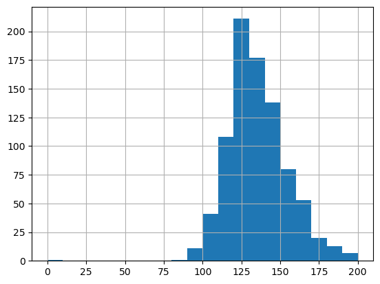
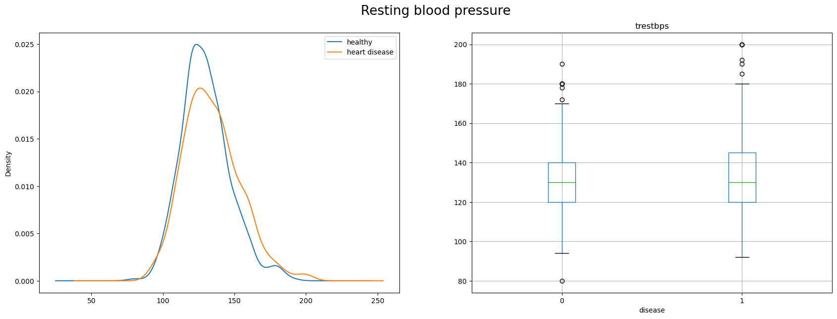
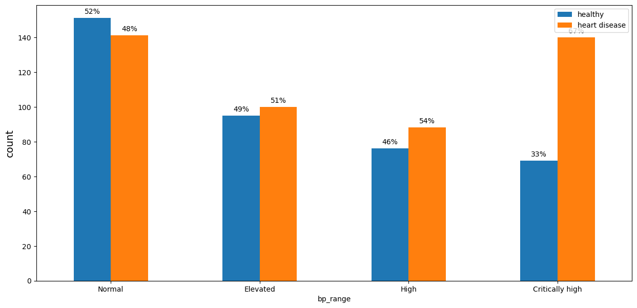
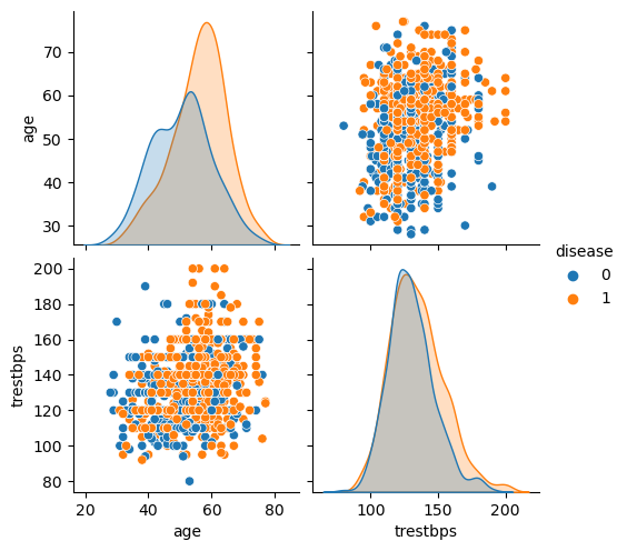
  • trestbps - resting blood pressure (in mm Hg on admission to the hospital)

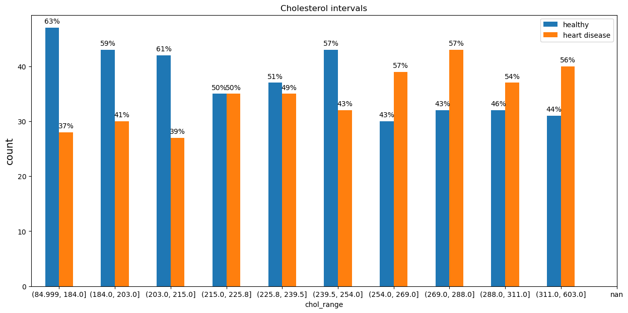
  • chol - cholesterol in mg/dl

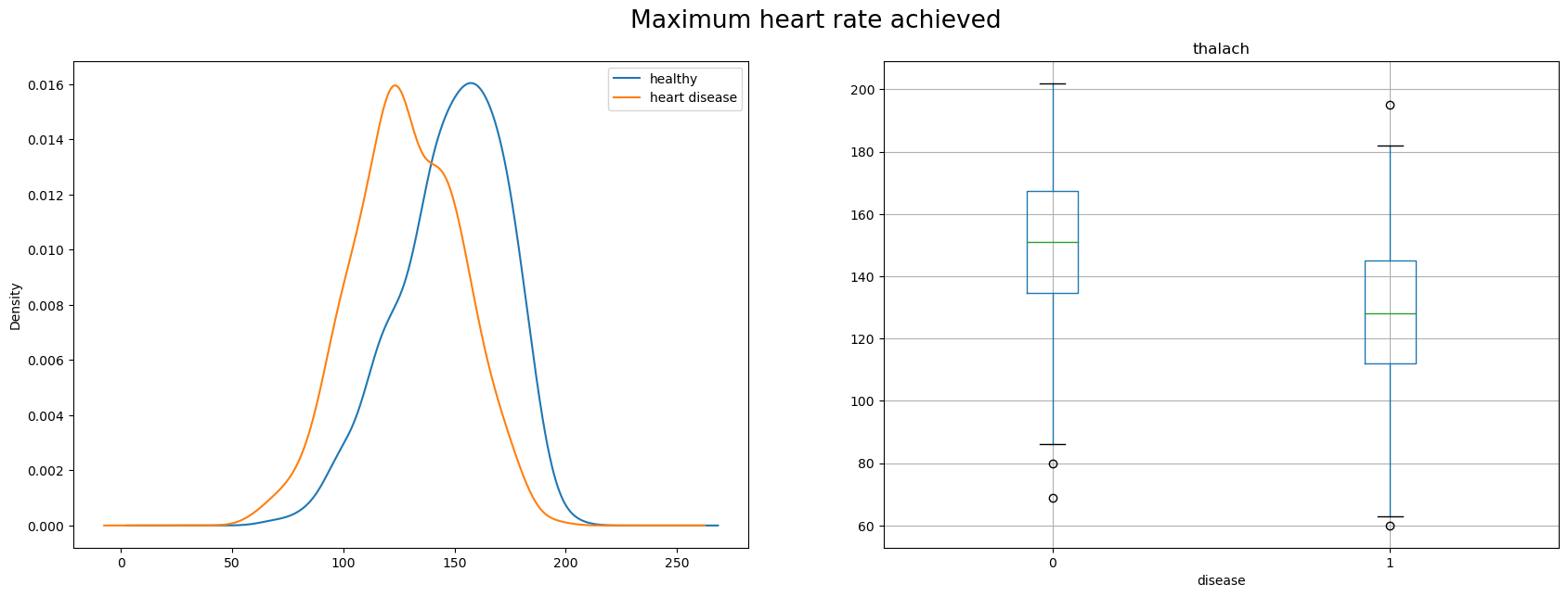
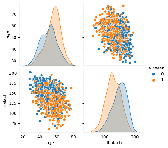
  • thalach - maximum heart rate achieved

  • oldpeak - ST depression induced by exercise relative to rest. ‘ST’ relates to the positions on the electrocardiographic (ECG) plot.

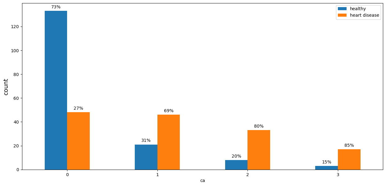
  • ca - number of major vessels (0-3) colored by flouroscopy. Fluoroscopy is one of the most popular non-invasive coronary artery disease diagnosis. It enables the doctor to see the flow of blood through the coronary arteries in order to evaluate the presence of arterial blockages.

Categorical attributes

  • sex: sex
    • 1 = male
    • 0 = female
  • cp: chest pain type
    • 1: typical angina
    • 2: atypical angina
    • 3: non-anginal pain
    • 4: asymptomatic
  • fbs - fasting blood sugar > 120 mg/dl
    • 1 = true
    • 0 = false
  • restecg - resting electrocardiographic (ECG) results
    • 0: normal
    • 1: having ST-T wave abnormality (T wave inversions and/or ST elevation or depression of > 0.05 mV)
    • 2: showing probable or definite left ventricular hypertrophy by Estes’ criteria
  • exang - exercise induced angina. Angina is a type of chest pain caused by reduced blood flow to the heart.
    • 1 - yes
    • 0 - no
  • slope - the slope of the peak exercise ST segment. (ECG)
    • 1: upsloping
    • 2: flat
    • 3: downsloping
  • thal - A blood disorder called thalassemia
    • 3: normal blood flow
    • 6: fixed defect (no blood flow in some part of the heart)
    • 7: reversable defect (a blood flow is observed but it is not normal)
  • disease - refers to the presence of heart disease in the patient. It is integer valued from 0 (no presence) to 4.

Exploratory data analysis

EDA helper functinos
df_eda = df.copy()

def plot_categorical(data=pd.DataFrame,
                     column=str,
                     labels=[],
                     target='disease',
                     target_labels=['healthy', 'heart disease'],
                     title='', font = 10, ax = None):
    crosstab = pd.crosstab(data[column], data[target])
    ax = crosstab.plot(kind='bar', figsize=(15, 7), rot = 0, fontsize=font, ax=ax)
    x = np.arange(len(labels))
    ax.set_xticks(x)
    ax.set_xticklabels(labels)
    ax.legend(target_labels)
    plt.ylabel("count", size=14)
    plt.title(title)

    bars =  ax.patches

    #compute percents
    total_by_category = crosstab.sum(axis=1)
    healthy_perc = round((crosstab[0] / total_by_category ) * 100)


    for (i, bar) in enumerate(bars):
      prc = healthy_perc.iloc[i] if i < len(healthy_perc) else 100 - healthy_perc.iloc[i % len(healthy_perc)]
      plt.annotate(str(int(prc)) + '%',
                    (bar.get_x() + bar.get_width() / 2., bar.get_height()),
                    ha='center', va='center',
                    xytext=(0, 9),
                    textcoords='offset points')


def plot_numeric(data=pd.DataFrame, column=str, title=str):
    fig, ax = plt.subplots(1, 2)
    fig.set_size_inches(20, 7)

    #with respect to the target
    healthy = data.loc[data.disease == 0, column]
    sick = data.loc[data.disease == 1, column]
    healthy.plot.density(ax=ax[0])
    sick.plot.density(ax=ax[0])
    ax[0].legend(['healthy', 'heart disease'])

    data.boxplot(by='disease', column= [column], ax=ax[1])

    fig.suptitle(title, fontsize = 19)


def describe_numeric(data=pd.DataFrame, column=str):
    temp = data[[column, 'disease']].copy()
    temp['healthy'] = data[data.disease == 0][column]
    temp['sick'] = data[data.disease == 1][column]
    return temp[[column, 'healthy', 'sick']].describe()

def plot_missing(data = pd.DataFrame):
  na_values_percent = data.isna().sum().sort_values(ascending=False) \
    .apply(lambda x: (x, round(x / data.index.size * 100, 2))) # (count, %)
  na_values_percent.apply(lambda x: x[1]).plot.bar() # (plot %)
  plt.ylabel("Percentage", size=14)
  plt.title('Missing values')

Numeric data summary

Code
df_numeric=df_eda.loc[:,['age','trestbps','chol','thalach','oldpeak']]
df_numeric.describe()
age trestbps chol thalach oldpeak
count 920.000000 861.000000 890.000000 865.000000 858.000000
mean 53.510870 132.132404 199.130337 137.545665 0.878788
std 9.424685 19.066070 110.780810 25.926276 1.091226
min 28.000000 0.000000 0.000000 60.000000 -2.600000
25% 47.000000 120.000000 175.000000 120.000000 0.000000
50% 54.000000 130.000000 223.000000 140.000000 0.500000
75% 60.000000 140.000000 268.000000 157.000000 1.500000
max 77.000000 200.000000 603.000000 202.000000 6.200000
Code
dcorr=df_numeric.corr(method='pearson')
sns.heatmap(data=dcorr,annot=True,fmt=".2f")
<AxesSubplot: >

Categorical data summary

Code
plt.figure(figsize=(5,5),dpi=200)
for (i, col) in enumerate(['sex','cp','fbs','restecg','exang', 'disease', 'thal', 'slope']):
  plt.subplot(3,3,i+1)
  df_eda[col].value_counts().sort_index().plot(kind='pie', figsize=(7,5), autopct='%1.1f%%', title = col, textprops={'fontsize': 5})

Analysing risk factors for heart disease

Cholesterol (‘chol’)

Cholesterol has a lot of 0 values, which is not possible.

Code
df_eda.chol.hist(bins=20)
df_eda['chol'] = df_eda['chol'].replace({0:np.nan})

Analysis

People with heart disease on average have a higher cholesterol level.

Code
plot_numeric(df_eda, 'chol', 'Cholesterol')

Code
describe_numeric(df_eda, 'chol')
chol healthy sick
count 718.000000 372.000000 346.000000
mean 246.832869 240.158602 254.008671
std 58.527062 55.767559 60.620439
min 85.000000 85.000000 100.000000
25% 210.000000 204.000000 216.000000
50% 239.500000 233.000000 248.000000
75% 276.750000 270.250000 284.750000
max 603.000000 564.000000 603.000000

Binning shows that people with cholesterol level more than 254 mg/dl have more than 50% chance of having a heart disease.

Code
df_eda['chol_range'] = pd.qcut(df_eda['chol'], 10, duplicates = 'drop')
plot_categorical(df_eda, 'chol_range', df_eda.chol_range.unique().sort_values(), title = 'Cholesterol intervals')

Age

People with heart disease on average are about 5 years older than healthy people.

Code
df_eda.age.hist(bins=20)
<AxesSubplot: >

Code
describe_numeric(df_eda, 'age')
age healthy sick
count 920.000000 411.000000 509.000000
mean 53.510870 50.547445 55.903733
std 9.424685 9.433700 8.718959
min 28.000000 28.000000 31.000000
25% 47.000000 43.000000 51.000000
50% 54.000000 51.000000 57.000000
75% 60.000000 57.000000 62.000000
max 77.000000 76.000000 77.000000
Code
plot_numeric(df_eda, 'age', 'age')

We can see that the risk of getting heart disease increases after the age of 54.

Code
df_eda['age_range'] = pd.qcut(df_eda['age'], 10)
plot_categorical(df_eda, 'age_range', df_eda.age_range.unique().sort_values())

Resting blood pressure (‘trestbps’)

Code
df_eda.trestbps.hist(bins=20)
<AxesSubplot: >

There’s one unrealistic value of 0, I replace it with na for analysis.

Code
df_eda.trestbps.replace({0:np.nan}, inplace=True)

People with heart disease on average have a slightly higher blood pressure than healthy patients.

Code
plot_numeric(df_eda, 'trestbps', 'Resting blood pressure')

Code
describe_numeric(df_eda, 'trestbps')
trestbps healthy sick
count 860.000000 391.000000 469.000000
mean 132.286047 129.913043 134.264392
std 18.536175 16.869867 19.617889
min 80.000000 80.000000 92.000000
25% 120.000000 120.000000 120.000000
50% 130.000000 130.000000 130.000000
75% 140.000000 140.000000 145.000000
max 200.000000 190.000000 200.000000

Most patients with normal blood pressure do not have heart disease, while most patients with elevated blood pressure have heart disease.

Code
bins = [0, 120, 130, 140, np.inf]
labels = ['Normal', 'Elevated', 'High', 'Critically high']
df_eda['bp_range'] = pd.cut(df_eda['trestbps'], bins)
plot_categorical(df_eda, 'bp_range', labels)

Exercise induced angina (‘exang’)

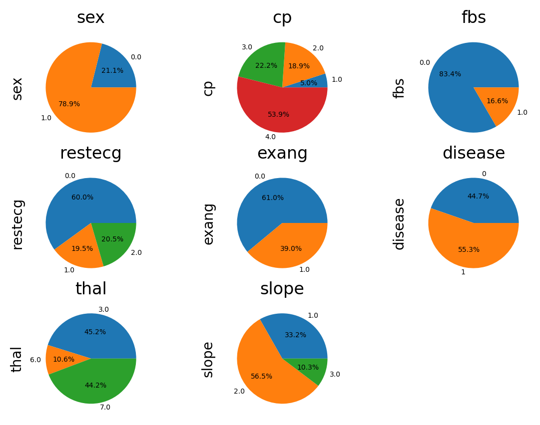
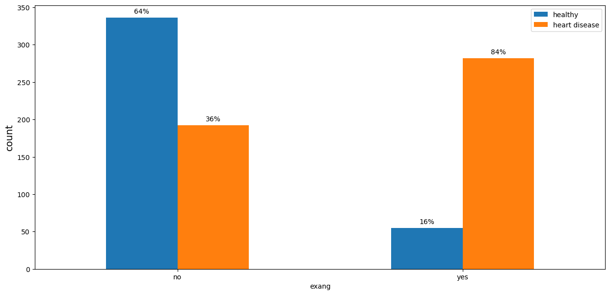
Most of the patients with heart disease experienced angina during the exercise, while the majority in the healthy group had no such symptoms.

Code
plot_categorical(df_eda, 'exang', ['no', 'yes'])

Number of Blocked Vessels (‘ca’)

The chance of having heart disease increases proportionally to the number of blocked vessels. Patients with 0 blocked vessels have only 27% chance of having heart disease. The value reaches 85% chance for the group with 3 blocked vessels.

Code
labels=["0", "1", "2", "3"]
plot_categorical(df_eda, 'ca', labels)

Gender

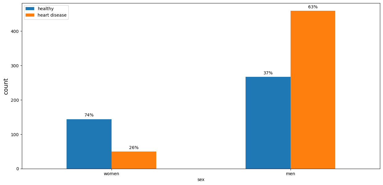
The majority of men in the dataset have heart disease, while only 26% of women are unhealthy.

Code
plot_categorical(df_eda, 'sex', ['women', 'men'])

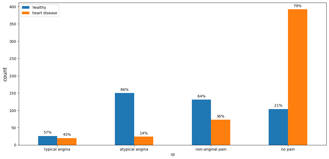
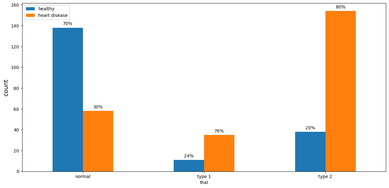
Chest pain type (‘cp’)

Amongst the patients with no chest pain almost 80% had heart disease. Patients with the atypical angina had the lowest level of heart disease rate. Overall, we can not say if a chest pain can be considered as a risk factor for a heart disease.

Code
labels=['typical angina', 'atypical angina', 'non-anginal pain', 'no pain']
plot_categorical(df_eda, 'cp', labels)

Fasting blood sugar

In the dataset most people don’t have a high sugar level. But among those who do, almost 70% have heart disease.

Code
plot_categorical(df_eda, 'fbs', ['Normal', 'High'])

Resting electrocardiographic results (‘restecg’)

Patients in the categories with type 1 and type 2 abnormalities have higher chance of getting a heart disease than the group with normal ECG.

Code
labels=['normal', 'type 1', 'type 2']
plot_categorical(df_eda, 'restecg', labels)

Maximum heart rate achieved (‘thalach’)

Code
df_eda.thalach.plot.hist(bins=20)
<AxesSubplot: ylabel='Frequency'>

Patients without heart disease are able to reach a higher maximum heart rate than patients with the disease.

Code
plot_numeric(df_eda, 'thalach', 'Maximum heart rate achieved')

ST depression (oldpeak)

Code
df_eda.oldpeak.hist()
<AxesSubplot: >

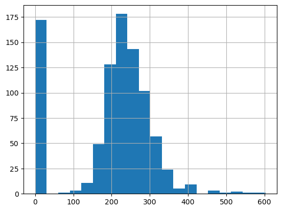
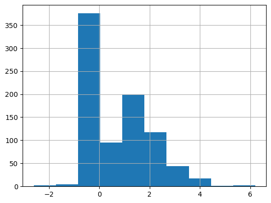
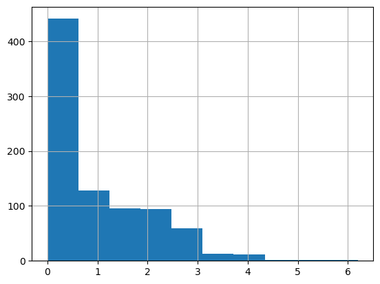
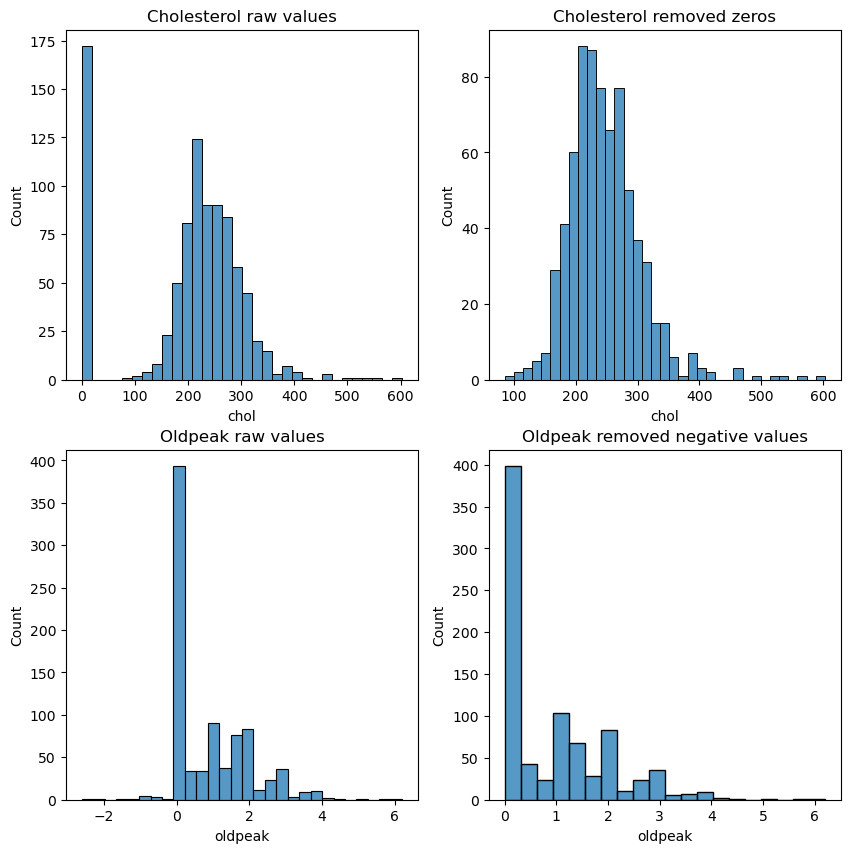
There are some negative values. Replacing with nan.

Code
df_eda['oldpeak'] = df_eda['oldpeak'].apply(lambda x: np.nan if x < 0 else x)
df_eda.oldpeak.hist()
<AxesSubplot: >

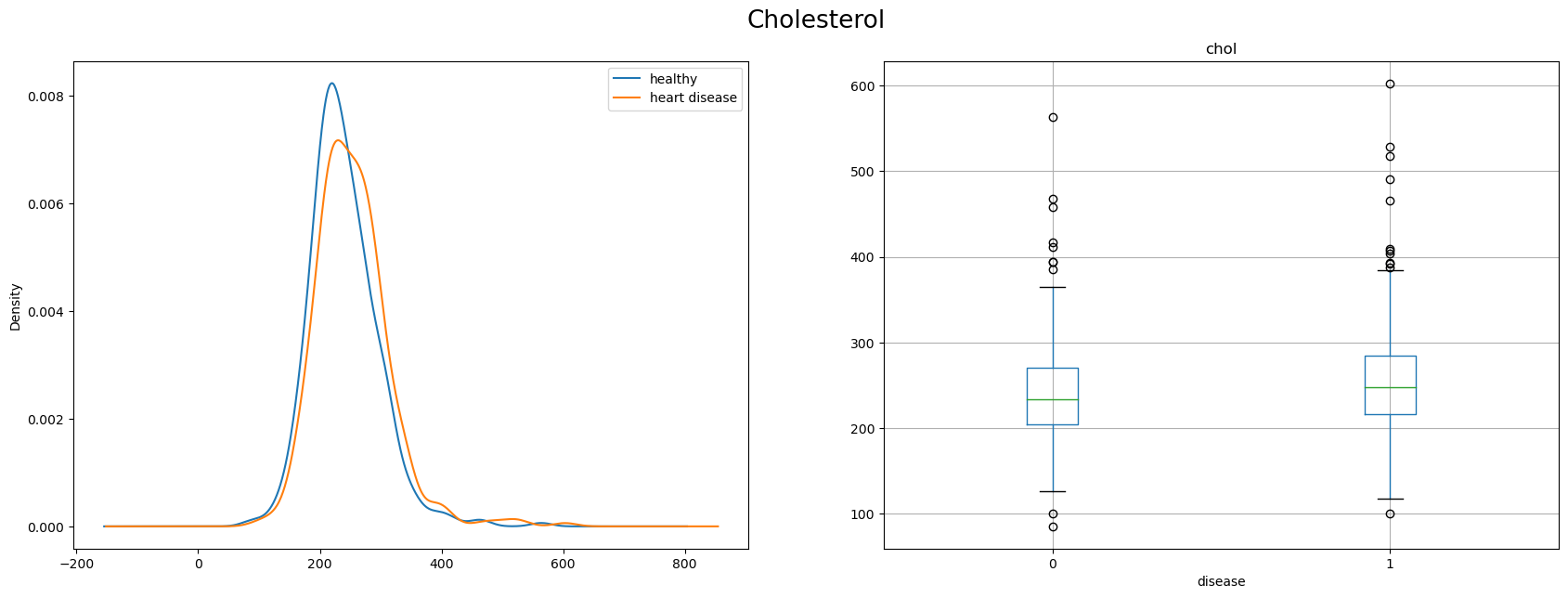
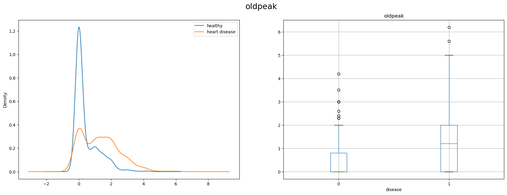
Oldpeak is another ECG parameter measuring ST depression during the exercise. It represents a distance on the ECG plot between specific points. There’s a notable difference in distributions between the groups. Sick people on average have higher value of the parameter.

Code
plot_numeric(df_eda, 'oldpeak', 'oldpeak')

Code
describe_numeric(df_eda, 'oldpeak')
oldpeak healthy sick
count 846.000000 387.000000 459.000000
mean 0.906265 0.425840 1.311329
std 1.071192 0.712184 1.153295
min 0.000000 0.000000 0.000000
25% 0.000000 0.000000 0.000000
50% 0.500000 0.000000 1.200000
75% 1.500000 0.800000 2.000000
max 6.200000 4.200000 6.200000

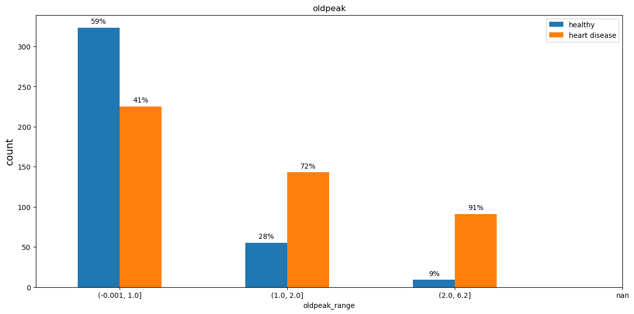
Patients with high olpeak values have higher chance of having herat disease.

Code
df_eda['oldpeak_range'] = pd.qcut(df_eda['oldpeak'], 5, duplicates = 'drop')
plot_categorical(df_eda, 'oldpeak_range', df_eda.oldpeak_range.unique().sort_values(), title = 'oldpeak')

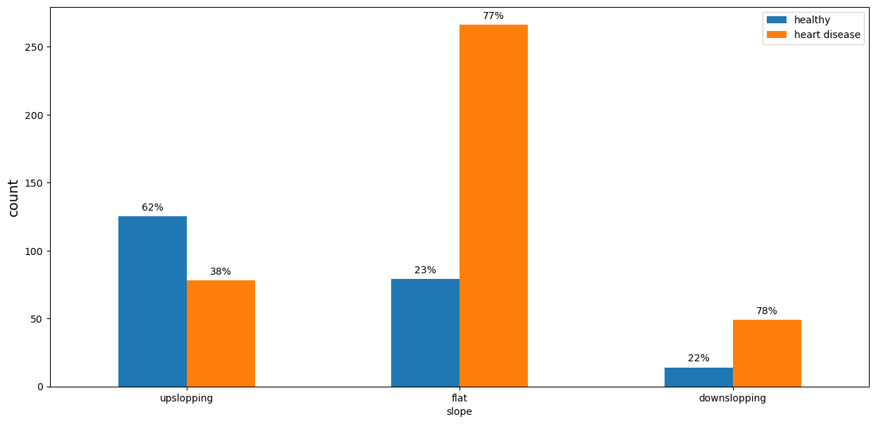
The slope of the peak exercise ST segment (‘slope’)

This is another ECG parameter, measured during the exercise. Almost 80% of the patients with ‘flat’ or ‘downslopping’ slope parameter had heart disease. Most of the people with the ‘upslopping’ slope were healthy.

Code
labels=["upslopping", "flat", "downslopping"]
plot_categorical(df_eda, 'slope', labels)

Thalassemia blood disorder (‘thal’)

People with this blood disorder are at risk of having heart disease with almost 80% for both type 1 and type 2 disorders.

Code
labels=['normal','type 1','type 2']
plot_categorical(df_eda, 'thal', labels)

Numeric attributes relationships

Younger patients are able to achieve higher maximum heart rate. Patients with heart disease are older and have lower maximum heart rate.

Code
sns.pairplot(df_eda, hue='disease', vars=['age', 'thalach']);

Blood pressure is higher in older patients. But these factors do not form a clear separation between healthy and sick patients.

Code
sns.pairplot(df_eda, hue='disease', vars=['age', 'trestbps']);

EDA colclusion

Exploratory data analysis identified the following groups with a high risk of heart disease:

  • Patients with high cholesterol
  • Patients older than 54 years old
  • Male patients
  • Patients with high blood sugar
  • Patients with abnormalities in their ECG
  • Patient low maximum heart rate
  • Patients with high oldpeak value
  • Patients with slope that flat or downsloping
  • Patients with blocked heart vessels
  • Patients with thalassemia blood disorder
  • Patients with high blood pressure, more than 120 mmHg

Data quality

Incorrect values

There are some incorrect values in the dataset as it was discovered.

  • Cholesterol (‘chol’) has lots of zeros.
  • ST depression (‘oldpeak’) has some negative values. In the existing research this parameter is >= 0.
  • Resting blood pressure (‘trestbps’) has one zero value.

Missing values

Count incorrect values as missing values.

Code
df_missing = df.copy()
df_missing.chol = df.chol.replace({0:np.nan})
df_missing.trestbps = df.trestbps.replace({0:np.nan})
df_missing.loc[df.oldpeak < 0, 'oldpeak'] = np.nan

plot_missing(df_missing)

Data Preparation

Data cleaning

Removing incorrect values.

Code
def remove_incorrect(data=pd.DataFrame):
  copy=df.copy()
  copy.chol.replace(0,np.nan,inplace=True)
  copy.trestbps.replace(0,np.nan,inplace=True)
  copy.loc[copy['oldpeak'] < 0, "oldpeak"] = np.nan
  return copy

df_clean = remove_incorrect(df)

#plot the result
fig, axs = plt.subplots(2, 2, figsize=(10, 10))

#chol
sns.histplot(data=df, x="chol", ax = axs[0,0])
axs[0, 0].title.set_text('Cholesterol raw values')
sns.histplot(data=df_clean, x="chol", ax = axs[0,1])
axs[0, 1].title.set_text('Cholesterol removed zeros')

#oldpeak
sns.histplot(data=df, x="oldpeak", ax = axs[1,0])
axs[1, 0].title.set_text('Oldpeak raw values')
sns.histplot(data=df_clean, x="oldpeak", ax = axs[1,1])
axs[1, 1].title.set_text('Oldpeak removed negative values')

Deleting columns with more than 30% missing data

Code
df_reduced = df_clean.drop(['ca', 'thal', 'slope'],axis=1)
df_reduced.head(1)
age sex cp trestbps chol fbs restecg thalach exang oldpeak disease
0 32.0 1.0 1.0 95.0 NaN NaN 0.0 127.0 0.0 0.7 1

Removing duplicate rows.

Code
duplicates = df_reduced.loc[df_reduced.duplicated(), :] 
df_no_duplicates = df_reduced.drop_duplicates(keep='first') 
duplicates
age sex cp trestbps chol fbs restecg thalach exang oldpeak disease
613 58.0 1.0 3.0 150.0 219.0 0.0 1.0 118.0 1.0 0.0 1
728 49.0 0.0 2.0 110.0 NaN 0.0 0.0 160.0 0.0 0.0 0

Outliers

Code
def find_outliers(data=pd.DataFrame):
    return [col for col in data.columns if has_outliers(data[col])]

def get_box_limits(col=pd.Series):
    q1 = col.quantile(.25)
    q3 = col.quantile(.75)
    IQR = q3 - q1
    ll = q1 - (1.5*IQR)
    ul = q3 + (1.5*IQR)
    return (ll, ul)

def has_outliers(col=pd.Series):
    ll, ul = get_box_limits(col)
    upper_outliers = col[col > ul].count() > 0
    lower_outliers = col[col < ll].count() > 0
    return upper_outliers or lower_outliers

outliers_columns = find_outliers(df_no_duplicates[['age', 'trestbps', 'chol', 'thalach', 'oldpeak']])

fig, axs = plt.subplots(1, len(outliers_columns), figsize = (20, 7))
for (i, col) in enumerate(outliers_columns):
   df_no_duplicates[col].plot.box(ax = axs[i], fontsize = 18)

These values are real, and removing them might affect the modeling, so I keep them.

Statistical significance testing

The best resource about univariate and bivariate statistical analysis basics:

Chi square test for categorical data

Code
from pandas.core.strings.accessor import isna
from itertools import combinations
from scipy.stats import chi2_contingency

def test(col1=pd.Series, col2=pd.Series, alpha=float):
  data_cont=pd.crosstab(col1, col2)
  p_value = chi2_contingency(data_cont)[1]
  return p_value > alpha

def color_df(x):
  if x == True:
    return 'color: %s' % 'red'
  elif isna(x): return None
  else: return 'color: %s' % 'green'

def show_chi_square_results(data=pd.DataFrame):
  categorical = ['sex','cp','fbs','restecg','exang', 'disease']
  cmb = list(combinations(categorical, 2))

  chi_square_results_df = pd.DataFrame(index = categorical, columns = categorical)
  for c in cmb:
    res = test(data[c[0]], data[c[1]], 0.05)
    chi_square_results_df.loc[c[0], c[1]] = res
    chi_square_results_df.loc[c[1], c[0]] = res

  return chi_square_results_df.style.applymap(color_df)

show_chi_square_results(df_no_duplicates)
  sex cp fbs restecg exang disease
sex nan False False True False False
cp False nan True False False False
fbs False True nan False True False
restecg True False False nan False False
exang False False True False nan False
disease False False False False False nan

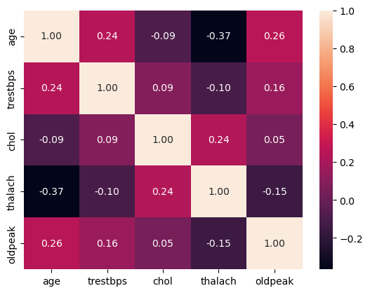
The table demonstrates if a variable is statistically independent from another variable(label ‘True’). There are no independent variables for the target (disease) column.

T-test for numeric features

Two-tailed two sample t-testing is performed.

Null Hypothesis: The means of features for patients with heart disease and healthy patients are the same.

Alternative hypothesis: There are statistically significant differences in the feature means for the healthy and sick patients.

Code
from scipy.stats import ttest_ind

def test_numeric(data = pd.DataFrame, col=str):
    data = data[~data[col].isna()]
    _, p = ttest_ind(data[col], data['disease'], equal_var=False)
    return p

def show_ttest_results(data=pd.DataFrame):
  results = [(col, test_numeric(data, col))  for col in ['chol', 'trestbps', 'age', 'oldpeak', 'thalach']]
  return pd.DataFrame(results, columns = ['Column', 'p-value'])
Code
show_ttest_results(df_no_duplicates)
Column p-value
0 chol 0.000000e+00
1 trestbps 0.000000e+00
2 age 0.000000e+00
3 oldpeak 9.389716e-19
4 thalach 0.000000e+00

I reject null hypothesis and state that there are statistically significant differences in the feature means for the healthy and sick patients. Keeping all the features.

Split train/test

70% train, 30% test

Code
train_data = df_no_duplicates.sample(frac=0.7, random_state=123)
test_data = df_no_duplicates[~df_no_duplicates.index.isin(train_data.index)]

Data imputation

Code
from scipy.stats import mode
from functools import partial

def impute(data,cols,impute_fn):
    imputed = data.copy()
    for col in cols:
        imputed[col + "_missing"] = imputed[col].isna().astype(int) # flag variable for missing 
        imputed[col] = impute_fn(imputed[col])#.fillna(imputed[col].mode()[0]) 
    return imputed

def impute_categorical(data=pd.DataFrame) -> pd.DataFrame:
    cols = ['restecg', 'exang', 'fbs']
    impute_fn = lambda x: x.fillna(x.mode()[0])
    return impute(data,cols,impute_fn)
    

def impute_numeric(data=pd.DataFrame, cols=list) -> pd.DataFrame:
    cols = ['oldpeak', 'trestbps', 'thalach', 'chol']
    impute_fn = lambda x: x.fillna(x.median())
    return impute(data,cols,impute_fn)

def plot_numeric_imputation(data_before=pd.DataFrame, data_after=pd.DataFrame):
  cols = ['oldpeak', 'trestbps', 'thalach', 'chol']
  fig, axs = plt.subplots(1, len(cols), figsize = (25, 5))
  for i, col in enumerate(cols):
    sns.kdeplot(data_before[col], color='b', fill=True, ax = axs[i], alpha = 0.07)
    sns.kdeplot(data_after[col], color='r', fill=True, ax = axs[i], alpha = 0.07)
    axs[i].legend(['Before imputation', 'After imputation'])

def plot_categorical_imputation(data_before=pd.DataFrame, data_after=pd.DataFrame):
  cols = ['restecg', 'exang', 'fbs']
  fig, axs = plt.subplots(1, len(cols), figsize = (25, 5))
  for i, col in enumerate(cols):
    sns.histplot(data=data_before, x=col, ax=axs[i], color='b')
    sns.histplot(data=data_after, x=col, ax=axs[i], color='r', alpha=0.2)
    
plot_numeric_imputation(train_data, impute_numeric(train_data))
plot_categorical_imputation(train_data, impute_categorical(train_data))

One hot encoding

Code
def encode_dummy(data = pd.DataFrame, drop_first=True) -> pd.DataFrame:
  df = data.copy()
  for col in ['cp', 'restecg']:
    dummy = pd.get_dummies(df[col], prefix = col,drop_first=drop_first)
    df = pd.concat([df, dummy], axis=1)
    df.drop(col, axis=1, inplace=True)
  return df

encode_dummy(train_data).head(5)
age sex trestbps chol fbs thalach exang oldpeak disease cp_2.0 cp_3.0 cp_4.0 restecg_1.0 restecg_2.0
349 47.0 1.0 112.0 204.0 0.0 143.0 0.0 0.1 0 0 0 1 0 0
654 38.0 1.0 140.0 297.0 0.0 150.0 0.0 0.0 0 1 0 0 0 0
7 38.0 1.0 115.0 NaN 0.0 128.0 1.0 0.0 1 0 1 0 0 0
571 54.0 1.0 NaN 182.0 0.0 NaN NaN NaN 0 1 0 0 1 0
171 65.0 0.0 140.0 417.0 1.0 157.0 0.0 0.8 0 0 1 0 0 1

Feature Scaling

Normalization/Standardization

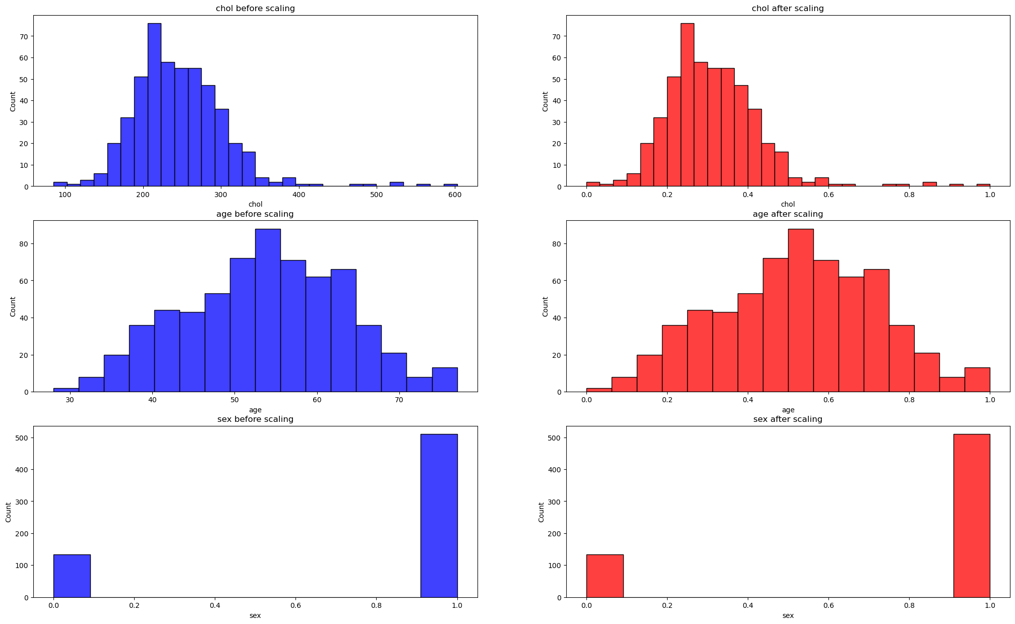
Machine learning algorithms like linear regression, logistic regression, neural network, etc. that use gradient descent as an optimization technique require data to be scaled.
Distance algorithms like KNN, K-means, and SVM are most affected by the range of features Normalization/Standardization.Therefore, I scale the data before employing a distance based algorithm so that all the features contribute equally to the result.

Code
from sklearn.preprocessing import MinMaxScaler

def scale(data=pd.DataFrame):
  return pd.DataFrame(MinMaxScaler().fit_transform(data), columns=data.columns)

def plot_normalization(data_before=pd.DataFrame, data_after=pd.DataFrame, cols=str):
  fig, axs = plt.subplots(len(cols), 2, figsize = (25, 15))
  for i, col in enumerate(cols):
    sns.histplot(data_before[col], color='b', ax = axs[i, 0])
    axs[i, 0].title.set_text(col + ' before scaling')
    sns.histplot(data_after[col], color='r', ax = axs[i, 1])
    axs[i, 1].title.set_text(col + ' after scaling')

plot_normalization(train_data, scale(train_data), ['chol', 'age', 'sex'])

Modeling

Helper functions
from sklearn.ensemble import RandomForestClassifier, RandomForestRegressor
from sklearn.model_selection import train_test_split
from sklearn.metrics import accuracy_score
from sklearn.linear_model import LogisticRegression

def run_modeling(model,train_data,test_data):
    x_train = train_data.drop('disease', axis=1)
    y_train = train_data['disease']
    model.fit(x_train, y_train)
      
    x_test = test_data.drop('disease', axis=1)
    y_test = test_data['disease']
    y_model = model.predict(x_test)
    return accuracy_score(y_test, y_model), model


def impute_all(data):
    return impute_categorical(impute_numeric(data))

def full_pipeline(data):
    data = impute_all(data)
    data = encode_dummy(data)
    return scale(data)

Random forest

rf_train_data  = impute_all(train_data)
rf_test_data  = impute_all(test_data)

acc, rf_model = run_modeling(RandomForestClassifier(random_state=0), rf_train_data,rf_test_data)
print(f'accuracy: {acc}')
accuracy: 0.7527272727272727

Logistic regression

lr_train_data = full_pipeline(train_data)
lr_test_data = full_pipeline(test_data)
    

acc, model = run_modeling(LogisticRegression(), lr_train_data, lr_test_data)
print(f'accuracy: {acc}')
accuracy: 0.7781818181818182

SVM

There are many model parameters and they are not easy to choose, so I use the GridSearchCV tool in sklearn to help to complete the parameter selection. The main parameters include kernel, C and gamma

from sklearn import svm
from sklearn.model_selection import GridSearchCV

parameters = {'kernel':('linear', 'rbf'), 'C':[1], 'gamma':[0.05, 0.07, 0.125, 0.25, 0.5]}
model = GridSearchCV(svm.SVC(), parameters, scoring='accuracy')

svm_train_data = full_pipeline(train_data)
svm_test_data = full_pipeline(test_data)

acc, model = run_modeling(model, svm_train_data, svm_test_data)
print(f'accuracy: {acc}')
accuracy: 0.7781818181818182

Interpretation

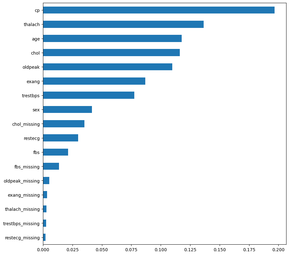
I use information from the random forest feature importance to do interpretation.

From the random forest feature importance information I conclude that the most important variables for predicting heart disease are:

  • Chest pain type (cp)
  • Maximum heart rate achieved (thalach)
  • Oldpeak
  • Age
  • Cholesterol

Meanwhile such parameters as blood sugar and the results of the electrocardiogram contributed the least to the heart disease prediction in the random forest model.

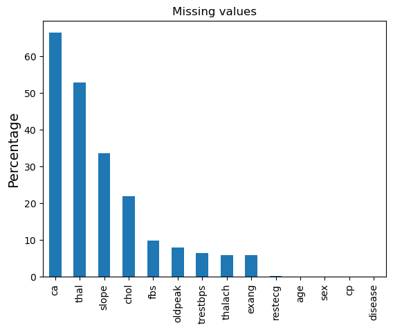
The most of the missing values flags were not important for the model.

Code
(pd.Series(rf_model.feature_importances_, index=rf_train_data.drop(['disease'], axis=1).columns).sort_values().plot(kind='barh', figsize=(10,10)))
<AxesSubplot: >