Gradient accumulation

Toy example for gradient accumulation understanding

One of the techniques which can be used to train bigger models with less GPU memory is gradient accumulation. It is a training technique where gradients computed during multiple mini-batches are accumulated before performing a weight update, effectively simulating larger batch sizes without the memory requirements.

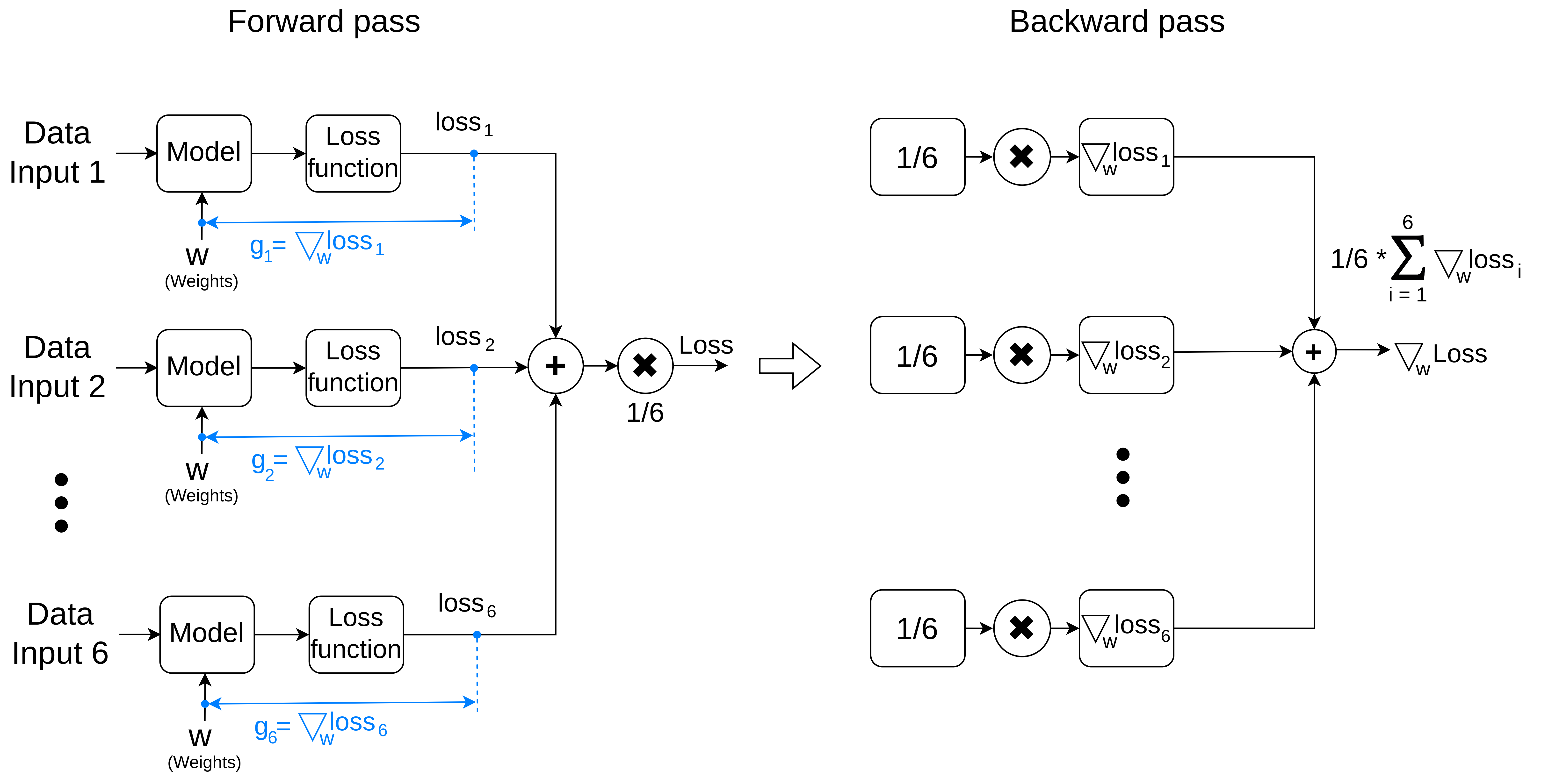
Given a model and a loss function, in the forward pass the final loss value is computed as an average of loss values for all samples in a batch. In a backward pass gradients are computed for each input and added together. Below is a diagram showing forward and backward passes for a batch of 6 items:

Computation without gradient accumulation

Let’s create a simple toy example with model performing only a dot product and an identity loss function

import torch

w = torch.randn(3)
x = torch.randn(6,3)

def forward(x,weights):
    return x@weights

weights = w.clone()
weights.requires_grad_(True)

# forward
batch = x
result = forward(batch,weights).mean()

#backward
result.backward()
weights.grad

tensor([-0.3536,  0.0207, -0.6125])

Gradient accumulation without normalization

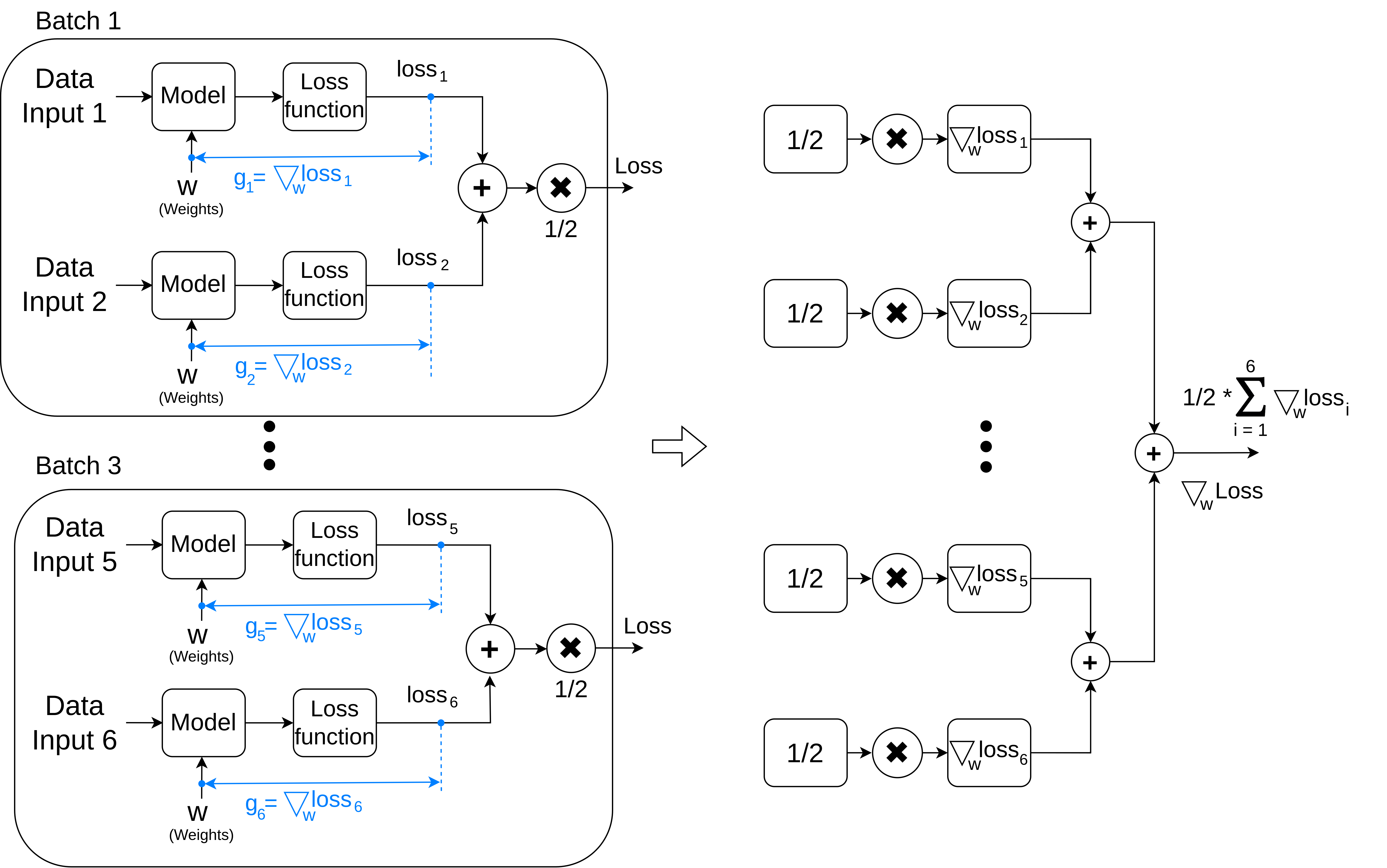
If we decide to distribute the computation into 3 batches of 2 items, the gradient would be different.

An example below shows the diagram of such scenario:

The gradient is different here:

weights = w.clone()
weights.requires_grad_(True)

batch_size=2
for batch_n in range(0,len(x),batch_size):
    batch = x[batch_n:batch_n+batch_size]
    result = forward(batch,weights).mean() 
    result.backward()

weights.grad

tensor([-1.0608,  0.0620, -1.8375])

Gradient accumulation with proper normalization

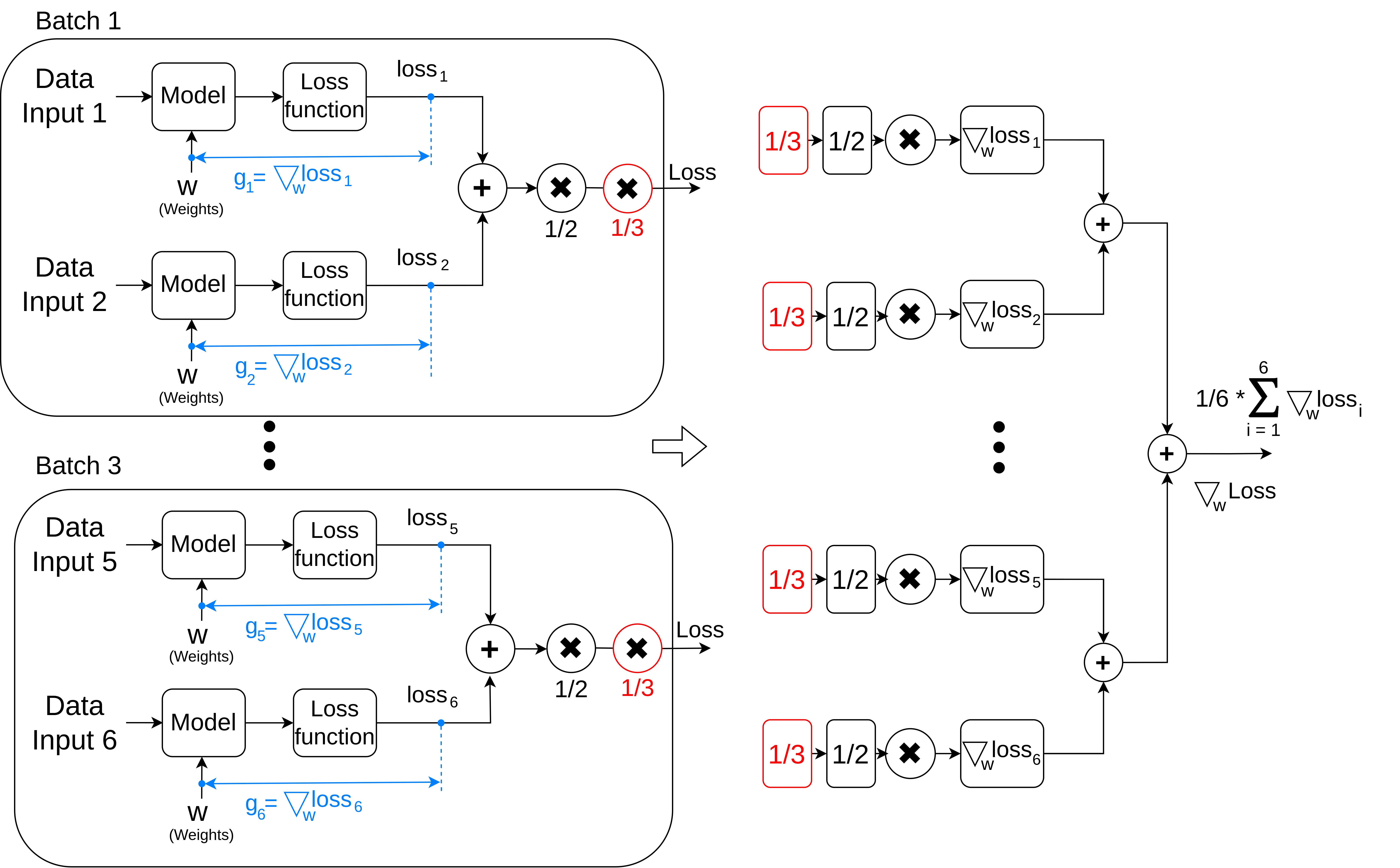
We can see that the reason for differences is the outcome are different normalization factors in the loss function. When we average loss values of each batch in isolation we don’t take into account the total amount of the items we want to accumulate gradients for. To correct the computation we need to add a normalization factor when computing a final loss value. This factor is a ratio between the total number of items we perform the computation for and the batch size. In our example it equals to \(6/2 = 3\)

The proper normalization produces correct gradient vector:

weights = w.clone()
weights.requires_grad_(True)

batch_size=2
for batch_n in range(0,len(x),batch_size):
    batch = x[batch_n:batch_n+batch_size]
    result = forward(batch,weights).mean() / 3
    result.backward()

weights.grad

tensor([-0.3536,  0.0207, -0.6125])

Practical implementation of this technique is well explained in the fast.ai course lecture.