Applying vision models to audio data

Fine-tuning ViTs and ConvNets on spectrogram data

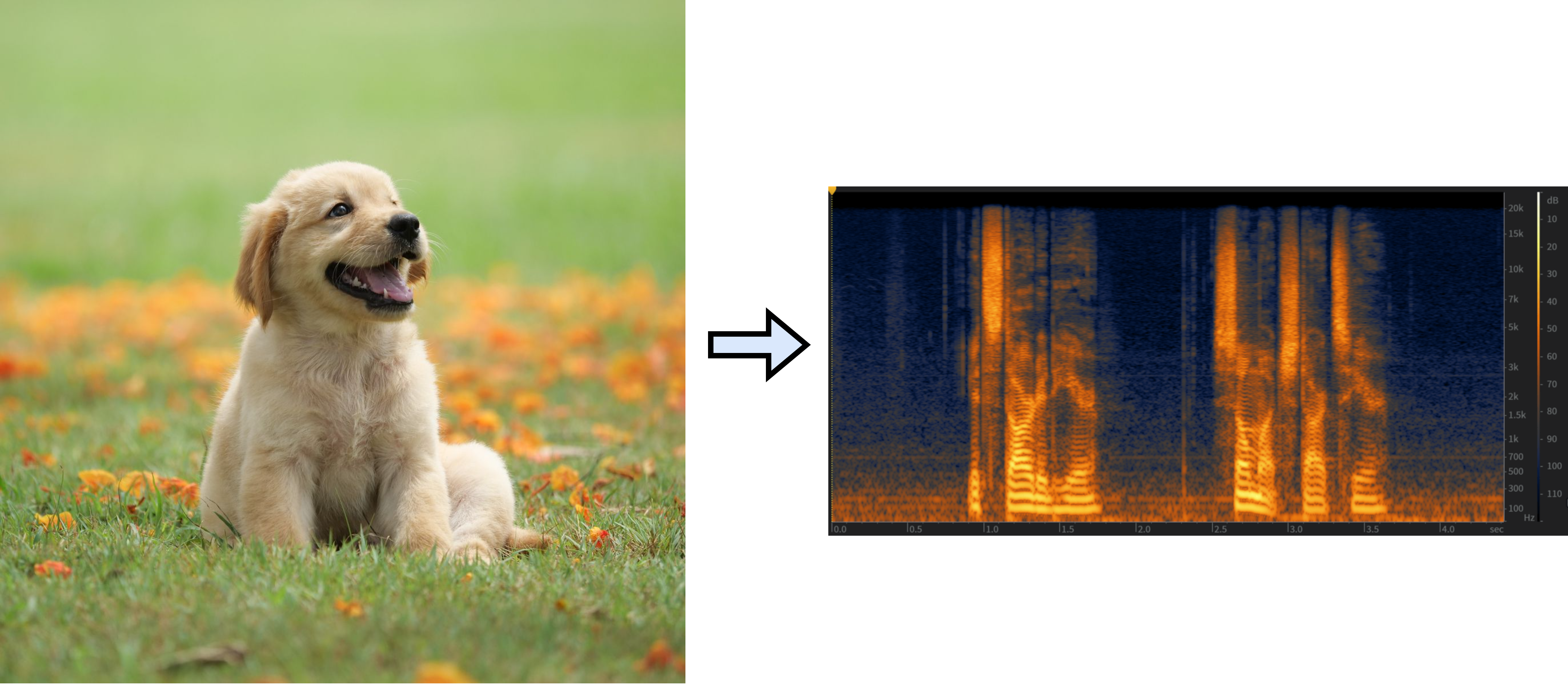
Several research have demonstrated that vision models pretrained on large datasets of images can be successfully applied for audio classification tasks. Both vision transformers and convolutional neural networks.

Vision transformers

The are 3 main modules in the vision transformer which are important for transfer learning:

The embedding module. Transforms images to a sequence of vector embeddings
Transformer encoder module. Contains stacked transformer encoder layers.
Head. Computes the final prediction from the obtained representation vector.

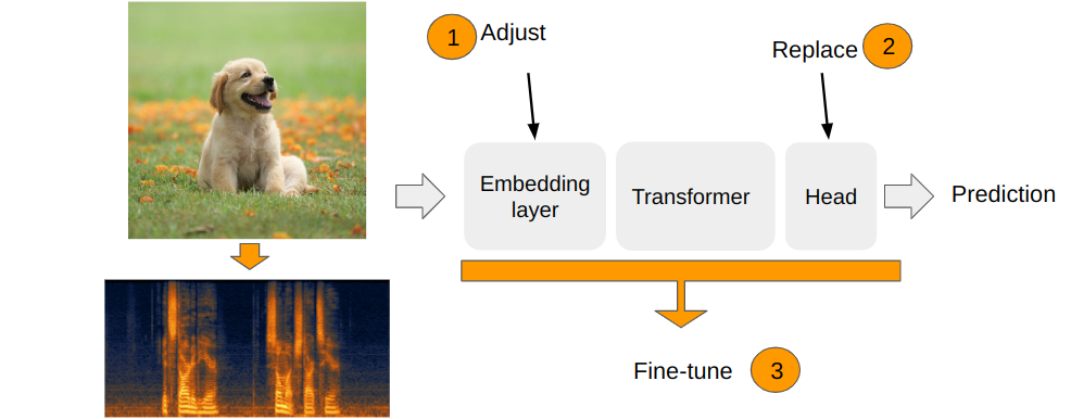
Adjusting the embedding layer

Embedding layer processing:

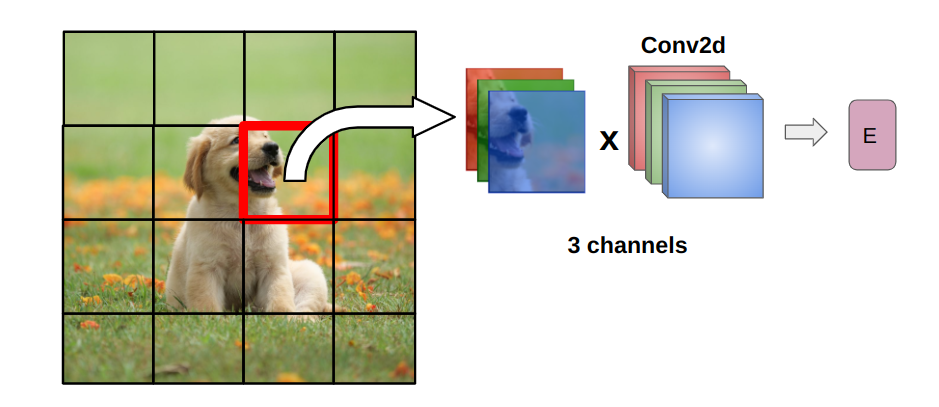
Split an image into patches
Compute patch embeddings
Add position encoding

Computing patch embeddings

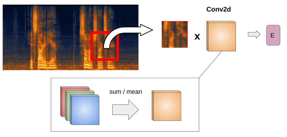
To compute an embedding from a patch, vision transformer applies a convolution operation with 3 input channels and the number of output channels equal to the specified embedding dimension.

Here’s how it is done in the timm library, from the timm.layers.PatchEmbed class:

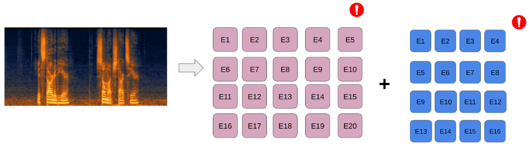
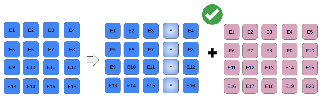
self.proj = nn.Conv2d(in_chans, embed_dim, kernel_size=patch_size, stride=patch_size, bias=bias)

When we work with spectrograms we have only 1 channel of information and that’s why the embeddings layer has to be adjusted.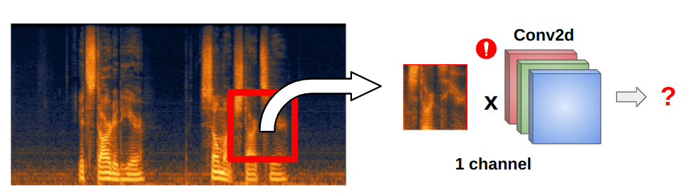

The adjustment can be done by copying spectrogram channel 2 times, averaging or taking a sum of the input channels of the embedding layer.

Timm library sums the weights of the convolution channels. From the adapt_input_conv function in the timm.models._manipulate:

conv_weight = conv_weight.sum(dim=1, keepdim=True)

The same is happening in the Audio Spectrogram Transformer:

new_proj.weight = torch.nn.Parameter(torch.sum(self.v.patch_embed.proj.weight, dim=1).unsqueeze(1))

Adjusting position embeddings

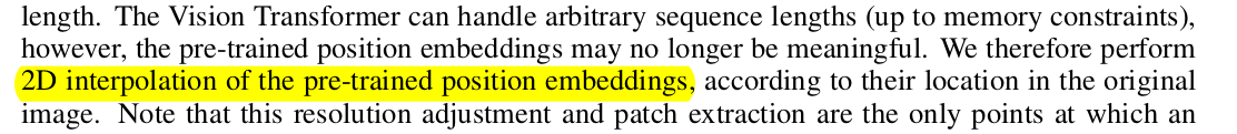
Position embeddings added to encode spatial information about the location of each patch in the image. Visual transformer models are pretrained on a fixed size images, which means they learn positional embeddings of a fixed size as well. To apply it to a different size images or spectrograms, position embeddings need to be somehow adjusted to transfer the learned relationships to different resolutions.

A popular solution - 2D interpolation.

From the original ViT paper, ‘Fine-tuning and higher resolution’ section:

Timm library also implements interpolation. From the github issue discussion:

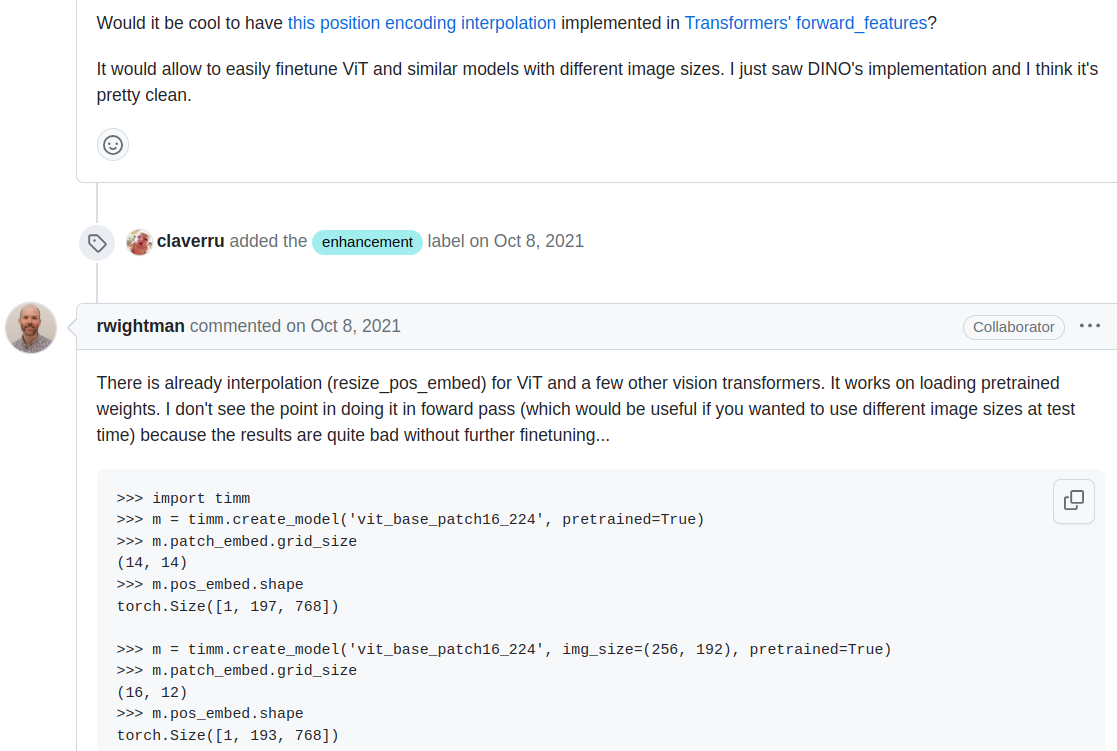
From the timm.layers._pos_embed.resample_abs_pos_embed:

posemb = F.interpolate(posemb, size=new_size, mode=interpolation, antialias=antialias)

Replacing the head

The final adjustment is simply changing the final layer for the specific task. The head layer in ViT consumes CLS token. So the new head should have the input dimension equal to the CLS token dimension (or just embeddings dimension).

* DeiT models have 2 CLS tokens, so there are 2 heads to adjust.

Example

Here’s how we can get a pretrained ViT model with adjusted embedding layer and the head layer for further fine-tunung:

m = timm.create_model('vit_base_patch16_224', img_size=size, pretrained=True, in_chans=1, num_classes=num_classes)

CNNs

For CNNs the process is mostly the same except they can work with variable size inputs, so we only need to adjust the number of input channels and the head. When we choose in_chans = 1 in timm library, under the hood adapt_input_conv function is called to adjust input layer as it was shown earlier:

conv_weight = conv_weight.sum(dim=1, keepdim=True)

m = timm.create_model('convnext_tiny', pretrained=True, in_chans=1, num_classes=num_classes)